About 2-3 years ago, Daphne Koller gave a thought-provoking talk on how representation learning can be used to accelerate drug discovery using genetics at the Big Data Institute, Oxford. I thought her talk was super cool as I also work on representation learning. But I couldn’t really understand what’s been done due to my lack of knowledge in the field of genetics. Thus, I decided to write on this topic to teach myself about the value of representation learning for genomic discovery.
Genetics, environmental exposure, and lifestyle are three pillars of human health. Due to recent advances in sequencing technologies, we can now sequence the human genome much faster and cheaper. The estimated cost of sequencing the first human genome sequencing is 300 million US dollars over 15 months in the Human Genome Project around the year 2000. Today, one can sequence their own DNA at a cost of a few hundred bucks within a few hours. Therefore, large volumes of human genome data have been collected for health discovery at a scale not possible before, such as the UK Biobank and Our Future Health initiatives.
The human genome roughly consists of 3 billion base pairs of nucleotides and 20K genes across 23 chromosomes. To make sense of the functions of each gene, we often deploy a statistical technique called genome-wide Association analysis (GWAS) by performing lots of logistic regressions to compare whether there are genetic differences across populations. The goal is to determine, for instance, whether populations that have variants of a gene have different body fat or risk of breast cancer. One of the very nice things about genetics is that because our genetic data largely stay unchanged since birth, we identify causal associations between our DNA and traits of interest. Making causal claims will be challenging in other types of observational studies as we will be subject to potential bias and confounding, which is a whole research topic on its own. If you want to know more about causal inference, the Book of Why by Judea Pearl will be a must-read.
Why representation learning?
Why does representation learning matter for genomic discovery? It matters because GWAS relies on converting the phenotyping measurement into a single scalar value. While the existing approach works for simple phenotypes like height and weight, it will be much more challenging to do so for high-dimensional cross-sectional data such as brain imaging and CT scans or low-dimensional high-frequency data such as wearable sensing data. I will refer to them as high-content clinical data. When performing GWAS on high-content clinical data, we have the following limitations:
- Huge reduction in dimensionality: In terms of raw data volume, modern measurement instruments can be high-dimensional. Using wearables as an example, one week of recording can lead to 10M+ data points, but we will have to condense this data sequence into a simple scalar value, such as weekly step count in a GWAS. Regardless of what magic number we come up with, the high degree of dimension reduction will lead to information loss. Even though we can perform the GWAS on every single dimension of the recorded sequence for 10M+ times, it will be computationally intractable.
- Reliance on expert-curated labels: Typically, the phenotype or trait of interest is defined by experts and often also has to be annotated by an expert. Inevitably, expert-defined labels will be limited in volume. So we won’t have enough power to detect the genetic variations that are less common.
- Missing features not discernable by humans: The high-content clinical data could have subtle features not discernable by humans. In wearable space again, when we look at traces of an accelerometer, it is difficult to know what activity someone is doing. Still, it will be possible to infer the activity being performed using data-driven approaches.
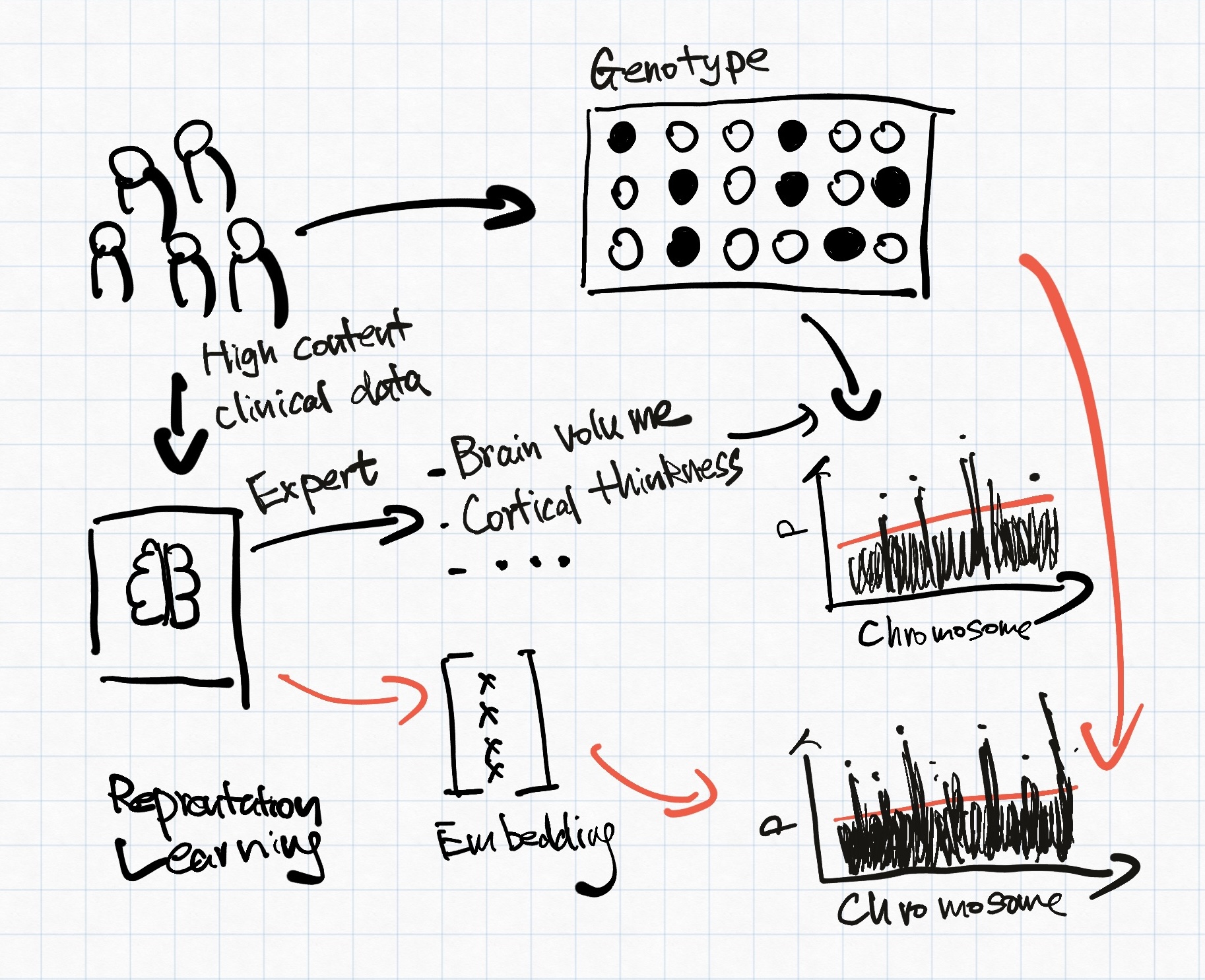
Representation learning has been investigated to address the issue above for a better-informed genomic discovery pipeline. Representation learning/feature learning describes a class of data-driven learning methods aiming to compress high-dimensional data into a lower-dimension latent space, sometimes referred to as embeddings. Principle component analysis (PCA) is a commonly used representation. However, PCA only captures linear relationships within its principle components, which is insufficient for high-dimensional clinical data. Figure 1 explains how representation learning-based phenotyping might differ from expert-curated phenotypes. For the rest of the blog post, we will explore how current representation learning methods can help with genomic discovery.
How to obtain the embeddings?
Current works mostly rely on using auto-encoder to minimise reconstruction loss. Alternatively, contrastive approaches have also been explored.
Reconstruction
REpresentation learning for Genetic discovery on Low-dimensional Embeddings (REGLE)
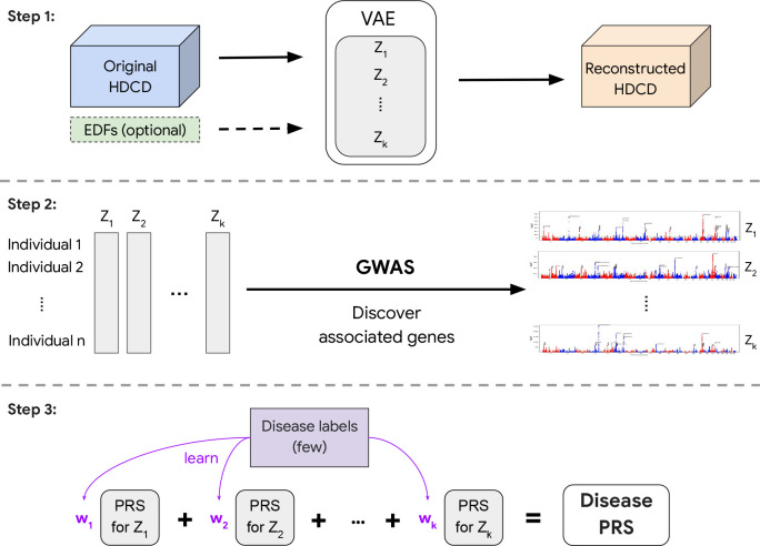
In 2023, Google published one of my favourite papers on phenotype representation learning using reconstruction. The authors proposed a generic framework called REpresentation learning for Genetic discovery on Low-dimensional Embeddings (REGLE). The study consists of three steps, shown in Figure 2:
- They learnt the embedding of high-content clinical data including photoplethysmography (PPG) for cardiovascular functions and spirograms for lung functions using variational autoencoder (VAE) as the backbone using reconstruction as the learning objective.
- GWAS was then performed on the obtained embeddings.
- Polygenic risk scores (PRS) were computed on each of the coordinates of the embeddings and then used to construct a disease-specific PRS.
What I like about this paper is that instead of using a normal autoencoder, they used VAE instead whose coordinates will be less coupled with each other. Having less correlated coordinates could enforce learning different aspects of the underlying biology.
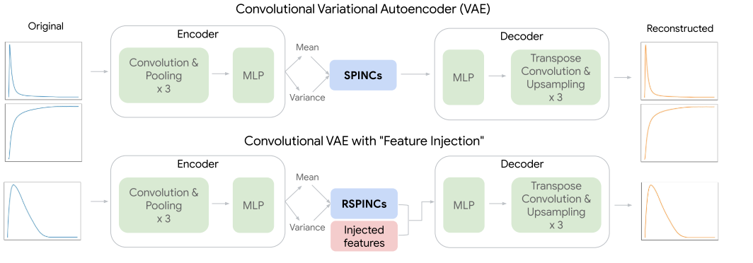
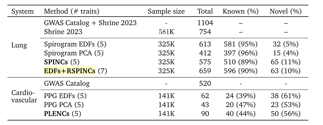
REGLE introduced three sets of embeddings, two for spirograms (SPINCs and EDFs+SPINCs) and one for PPG (PLENCs). For spirogram embedding, EDFs+SPINCs embedding set also had the EDFs information injected by feeding the EDFs to the decoder during reconstruction (Figure 2). The embedding-based approaches were able to discover more loci in general for both PPG and spirograms (Table 3). However, it is interesting to note that when embedding was learnt only on spirograms (SPINCs), fewer known loci (510) were discovered than when using the expert-defined phenotypes (581). Not sure if it is because of the larger sample size of spirograms. Perhaps this motivated the authors to add EDFs into the embedding learning to eventually discover greater known loci (596) alone.
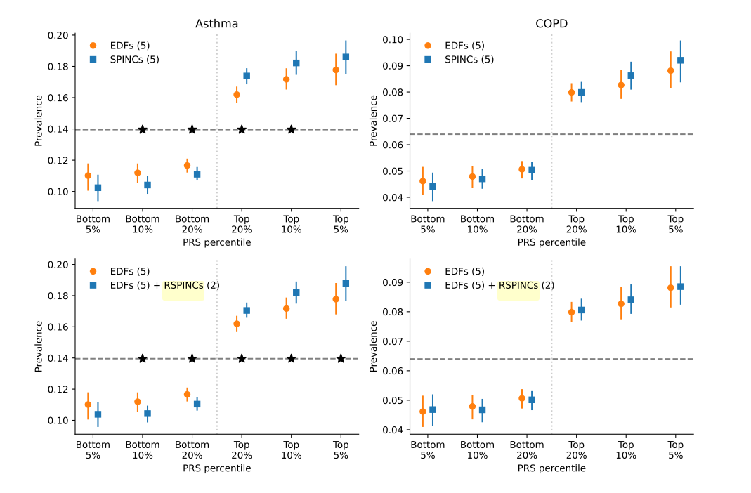
To compare disease-relevant polygenic risk scores (PRS) for different phenotypes, EDFs, and PPG or spirogram embeddings, a set of intermediate PRSes were first computed against each coordinate of the embeddings or pre-defined trait in EDFs. PRS for each coordinate can then be regressed against the target disease. Indeed, as shown in Figure 3, embedding-based PRSs can better stratify disease prevalence at different PRS percentiles. It seems a bit hard to interpret how much better the embedding-driven PRS is. Whether the enhanced stratification makes a meaningful difference in PRS depends on the heritability of each disease and whether we are sufficiently powered for the GWAS.
Optical Coherence Tomography autoencoder
Concurrently, two other studies, Optical Coherence Tomogrpahy (OCT) autoencoder and Unsupervised Deep Learning derived Imaging Phenotypes (UDIPs), tried to use autoencoders instead of VAEs as the backbones to learn the embeddings. We’ll use OCT autoencoder to illustrate how autoencoder-based embedding might differ from VAE-based embedding.
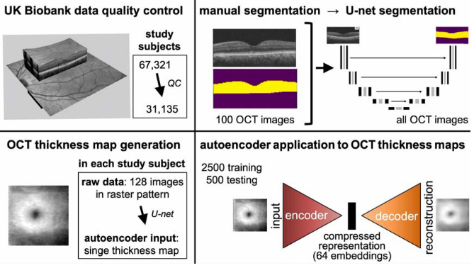
The OCT autoencoder paper also used data from the UK Biobank. OCT is a non-invasive imaging technique for the cross-sectional view of the human retina. Each OCT scan contains 128 cross-sectional images of the retina. A U-net was first trained on a set of 100 OCT scans that had manual segmentation maps to obtain an OCT thickness map generator. The retinal thickness maps of the left eye were used to obtain an embedding of 64 coordinates using the autoencoder (Figure 4). The OCT embedding was much larger than the PPG and spirogram embedding used in the REGLE paper (5-7 coordinates) to perhaps account for the increase in data volume.
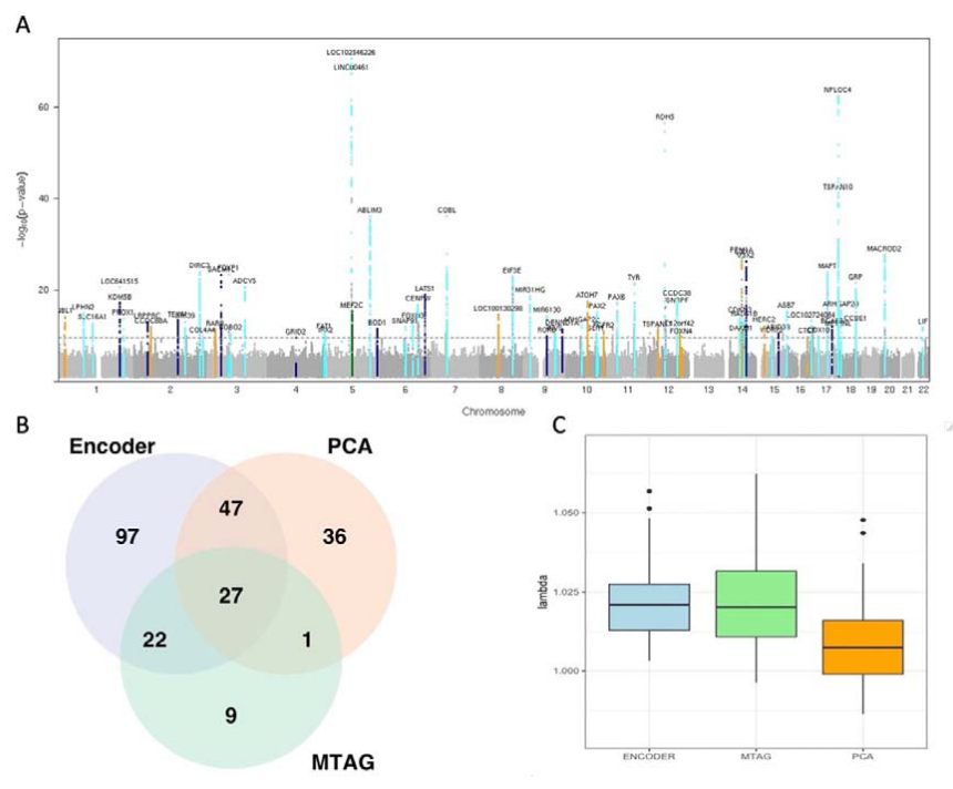
Since the autoencoder-based embeddings were correlated, the authors performed GWAS on the embeddings, but also the first 25 principal components of the embeddings, and a multi-trait meta-analysis (MTAG), a computationally efficient method to jointly analyze multiple related traits (Figure 5). In total, 239 lead loci were identified, 118 of which remained significant following Bonferroni correction. The authors reserved a subset of the UK Biobank participants for replication analysis. A total of 17 loci were replicated in the end, most of which were linked to the retinal layer thickness parameters. To further demonstrate the utility of the embeddings, the authors further used survival analysis to describe the predictive value of the embeddings and how the embeddings can be used for risk stratification of diseases.
Contrastive learning
Distinct from reconstruction, contrastive learning obtains the embeddings by learning representations that are invariant to simple transformations. The model aims to represent different views of an input in a similar way.
Image-based genome-wide association study
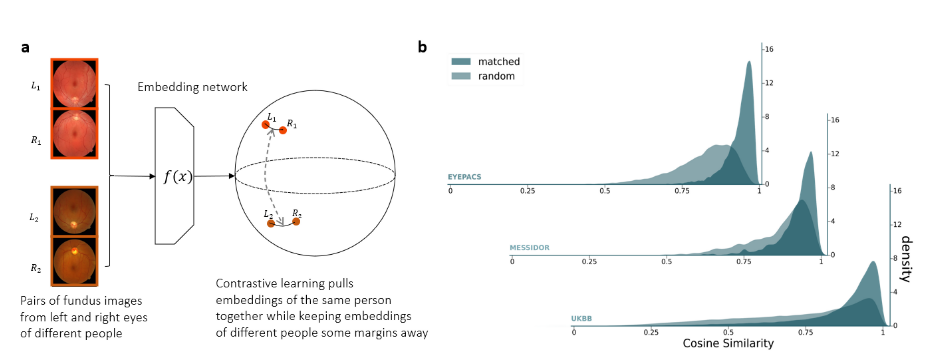
The image-based genome-wide association study (iGWAS) obtained its embeddings for retinal fundus photos capturing structure information regarding the retina, optic disc and macula from the back of the eye. The retinal fundus photos were first preprocessed into vessel segmentation masks. The embedding was trained on the segmentation masks using a modified version of ArcFace, an angular loss that maximises the distance between embeddings of different individuals while keeping the representations from the same individual close to each other (Figure 6.a). Specifically, the network was minimising the embedding distance between representations of the left and right retinas from the same individuals. Indeed, the cosine similarity is greater for matched retinas than random pairs in both the training dataset (EyePACS) and held-out test datasets (Messidor and UK Biobank) shown in Figure 6.b.
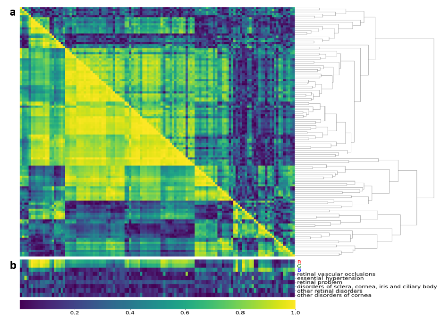
There are no benchmarks in comparing the embeddings produced by different machine learning methods. The embeddings obtained by contrastive learning have highly correlated clusters both on a phenotypical and genetic level (Figure 7.a). In particular, when assessing the embeddings with RGB values of the retina image, two clusters emerged. One cluster shows a high correlation with red and green values. And another cluster that has a greater correlation with the blue values. Given that the embeddings were designed to learn features related to vasculature, the structural arrangement of the retina, the embeddings should be invariant to the color of the retina. The authors admitted that better learning methods could alleviate the influence of retina color on the embedding space.
Among all the novel genes being identified using the embedding GWAS, the authors performed a functional follow-up for a novel gene WNT7B. The WNT7B has only been known to be important in the blood-brain barrier development and its role in the retinal vessels has not been identified. To confirm the role of WNT7B gene, the authors compare the differences in mouse retinas in vivo by knocking off the Wnt7B gene using the short hairpin RNA technique which can silence target gene expression via RNA interference. It turns out that when WNT7B was knocked down, the total vessel area increased significantly in the intermediate vascular plexus but reduced in the deep vascular plexus. This functional follow-up provides the first experimental evidence to validate the biological effect of embedding-based genomic discovery.
Cross-modal autoencoder
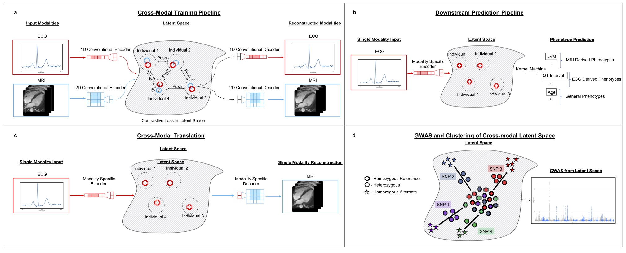
The final method that I want to cover here is a cross-modal embedding for the cardiovascular state. The cardiovascular state embedding was trained using cardio MRI and electrocardiogram (ECG) data, two complementary data modalities about the human heart. cross-modal, I think the authors want to imply that the modalities are paired and have knowledge transfer. Cross-modal learning is multi-modal but multi-modal learning might not be cross-modal. Even though the embedding of this paper was not directly used in the GWAS input, I still want to talk about some of its method considerations:
- The embedding was evaluated on three downstream tasks including phenotype prediction, imputation and genomic discovery.
- The embedding factors in information more than one modality.
- In the embedding-based GWAS, the effect of confounders was removed using iterative nullspace projection, which reduces the dimensionality of the latent space that can be used to predict the confounders.
Our results systematically integrate distinct diagnostic modalities into a common representation that better characterizes physiologic state
When it comes to the design of embeddings, one could either develop a representation optimised for every downstream task. Or one could develop a universal representation to be used for different types of downstream tasks. Given that we do have a single physical state for our organs like how the heart is the physical manifestation of our cardiovascular state and more. Intuitively, we should aim to develop a common representation if we have sufficient measurements to scale up the impact of the embeddings.
The objective function of the cross-modal embedding considers both reconstruction and contrastive loss as follows:
\[\begin{aligned} &\mathcal{L}\left(\left\{X^{(j)} f_j, g_j\right\}\right)=L_{\text {Contrast }}\left(\left\{X^{(j)}, f_j\right\}\right)+\lambda L_{\text {Reconstruct }}\left(\left\{X^{(j)}, f_j, g_j\right\}\right),\\ &L_{\text {Reconstruct }}\left(\left\{X^{(j)} f_j, g_j\right\}\right)=\sum_{i=1}^n \sum_{j=1}^m\left\|x^{(i, j)}-g_j\left(f_j\left(x^{(i, j)}\right)\right)\right\|^2,\\ &\begin{aligned} L_{\text {Contrast }}\left(\left\{X^{(j)} f_j\right\}\right)= & -\frac{1}{2} \sum_{I_k \in P_b} \sum_{j_1, j_2=1}^m \sum_{i=1}^{\left|j_k\right|} \log \left(\frac{\exp \left(e^{\text {temp }} f_{j_1}\left(x^{\left(i, j_1\right)}\right) \cdot f_{j_2}\left(x^{\left(i, j_2\right)}\right)\right)}{\sum_{i^{\prime}=1}^{\left|j_k\right|} \exp \left(e^{\text {temp }} f_{j_1}\left(x^{\left(i, j_1\right)}\right) \cdot f_{j_2}\left(x^{\left(i, j_2\right)}\right)\right)}\right) \\ & +\log \left(\frac{\exp \left(e^{\text {temp }} f_{j_1}\left(x^{\left(i, j_1\right)}\right) \cdot f_{j_2}\left(x^{\left(i, j_2\right)}\right)\right)}{\sum_{i^{\prime}=1}^{\left|j_k\right|} \exp \left(e^{\text {temp }} f_{j_1}\left(x^{\left(i, j_1\right)}\right) \cdot f_{j_2}\left(x^{\left(i, j_2\right)}\right)\right)}\right) \end{aligned} \end{aligned}\]Provided with input data with a subset of modalities \( X^{(i, j)}_{j\in\mathcal{I}} \), \( \mathcal{I} \in [m] \), where m is all the modalities available, we have an encoder \( f_j \) and a decoder \( g_j \).
\( L_{\text {Contrast }} \) aims to reconstruct the samples. \(L_{\text {Contrast }}\) makes sure data points from the same modalities of the same participant are similar. \( \lambda \) is used to balance the importance between the reconstruction loss and the contrastive loss.
Unlike previous studies for which the embeddings were directly used as the input for GWAS, the embeddings here were used to predict commonly used phenotypes such as the body-mass index and right ventricular ejection fraction to confirm it captures genotype-phenotype association for cardiovascular data. Not sure what the results might be if the GWAS was directly done on the embeddings.
Design choices
It’s not easy to read through the related work in representation learning for genomic discovery because the existing works have used different modalities, evaluation metrics and machine learning methods (Table 2). What’s clear though is that by using embeddings, it will be possible to move away from labeled datasets, have less dependency on expert-curated features and identify novel loci that might not be discovered using conventional techniques.
Also on a side note, I was amazed that the majority of the papers covered used data from the UK Biobank. Even though I work on the UK Biobank on a daily basis and so does everyone around me, it is incredible to see what people can do with rich resources like the UK Biobank on perhaps non-mainstream projects.
Table 2. Characteristics of phenotype representation learning
| Method | Learning objective | Model Architecture | Data source | Embedding Size | GWAS hits |
|---|---|---|---|---|---|
| REGLE | Reconstruction | Variational autoencoder | 170K PPG 351K spirograms |
5 | PPG: 40 known, 50 novel spirogram: 596 known, 63 novel |
| OCT autoencoder | Reconstruction | Autoencoder | 31K OCT images | 64 | 118: 17 were replicated |
| UDIP | Reconstruction | Autoencoder | 91K brain MRIs | 256 | 199: 145 novel |
| iGWAS | Contrastive | ConVNets | 105K fundus images | 128 | 34: 21 novel |
| Cross-modal autoencoder | Contrastive & Reconstruction | Autoencoder | 45K cardic MRIs, 39K ECG | 256 | NA |
I would want to highlight some of the key design choices that are important when developing the embedding for genomic discovery:
- Evaluation metric: Even though the end goal of the embedding, is to identify all the gene variants associated with a certain trait, Most of the embedding developed has not been evaluated for their usefulness for genomic discovery other than their training objectives. Metrics such as the heritability of an embedding, and relevance to diseases need to be assessed to develop the most relevant embedding (EmbedGEM)
- Scaling laws: By scaling laws, I am talking about the minimal amount of data and modal capacity needed to represent the state of our biology. For instance, in the cross-modal autoencoder paper, the network only had 10 million parameters to represent the cardiovascular state from cardiac MRIs and ECG data. If we are thinking about the complexity of the human heart, it seems a bit too small.
- Embedding size: Different modalities have different amounts of information. REGLE deliberately chose to smaller embedding space as the authors argued that it is better to have low-dimension uncorrelated embeddings and high-dimension correlated embeddings. Other approaches did not explicitly consider the influence of the embedding size w.r.t. the input information or the downstream GWAS.
- Learning paradigm: The machine learning techniques used thus far center around using autoencoder as the backbone with a reconstruction loss and contrastive loss. We don’t have any good data comparing the performance of different approaches.
- Universal representation: Ideally, we should be able to obtain a single encoder that generalises across populations. Having a universal representation will be computationally efficient as the users don’t need to obtain the embedding encoders on new datasets. Furthermore, the high-content clinical data measures some complex biology of the human body that has a universal representation in the real world.
Final thoughts
We are still in the early days of understanding the representation learning of the high-content clinical data for genomic discovery. As our measurement techniques, we will inevitably acquire richer high-content data in large volumes. Leveraging data-driven approaches to understand complex data modalities might help us understand our biology in a way not possible before.
Acknowledgment: I would love to thank the following people I chatted with on the ideas related to this post: Karl Simth, Nina Cai, Chris Nellåker, Chris Yau, Alkes Price, Angus Burns, Xilin Jiang, Steven Lin and Laura Portas.